Fun fact: Bayes’ Theorem, arguably one of the most important theorems in statistics, was discovered by Reverend Thomas Bayes, a Presbyterian minister/mathematician/theologian, and it was published posthumously thanks to Richard Price, a mathematician and Congregational minister. It should not come as a surprise, then, that it can be applied to questions at the fringe of Science and bear interesting results.

In particular, in this post I wanted to provide a simple introduction to Bayes’ Theorem and Bayesian Inference, and show some applications to supernatural phenomena; this weird choice of topic is motivated both by the alleged motivations behind the discovery of Bayes’ Theorem and by the fact that supernatural phenomena and theological problems are for a lot of people much more captivating than dice throws or other textbook ¹ examples. ¯\(ツ)/¯

Moreover, it will allow us to touch some really interesting topics about how Science progresses, and the apparent paradox of how rational people exposed to the same data can reach radically different conclusions.

I will start by writing some basic facts about probabilities and Bayes’ theorem; very likely the more experienced readers will be familiar with the content of the first sections, therefore I invite them to skip directly to the section Probing the Paranormal with Experiments

Full disclosure, since for many people this is a delicate argument: I do not believe in anything supernatural and I am not religious. I will try to avoid strawmanning positions different from mine, but I apologize in advance if I do, and please let me know what I got wrong by contacting me or in the comment section.

Probabilities and Experiments

Let’s start from an apparently elementary concept: the definition of probabilities. One way to define the probability of an event is to identify it as the limit of the relative frequency of that event with respect to every possible outcome, when the number of “experiments” tends to infinity.

For instance, if a coin is thrown \(100\) times and it lands \(57\) times on heads, the measured relative frequency of heads is \(57/100\). In order to obtain the probabilities associated with the throw of that coin, we need to calculate the limit of the relative frequency of heads in \(N\) throws as \(N\) grows infinitely. For a “fair” coin tossed in a “fair” way the probability of heads is, by definition, \(P_H = 1/2\) ².

This definition makes sense mathematically, but it leaves us with a problem: in order to know the probability of an outcome, we would need to perform an infinite amount of experiments. Since at the end of the day one can perform only a finite amount of experiments, people adopting this definition of probabilities, the so-called “frequentist interpretation”, mostly work with objects such as estimators and confidence intervals in order to extract as much information as possible from the finite number of samples one can obtain from experimental data.

Aside of the frequentist interpretation, there is another view of statistics which is called Bayesian interpretation. In order to understand it, we need to know some things about Bayes’ Theorem.

Bayes’ Theorem and Bayesian Inference

The probability of an outcome \(A\) assuming another event \(B\) happened is called a conditional probability, and is typically written as \(P(A|B)\). For definiteness, let’s consider a fair die; we know that the probability of throwing it and getting a \(1\) is \(P(\text{Die throw} = 1) = 1/6\). If a friend throws a fair die and tells us only that they obtain an odd number, in order to calculate the probability that they got a \(1\) without discarding the information they gave us we would use the conditional probability \(P(\text{Die throw} = 1 | \text{Die throw is odd})\).

Conditional probabilities are defined as:

\[P(A|B) = \frac{P(A \text{ and } B)}{P(B)};\]

thus, for the example I just gave, \(P(\text{Die throw} = 1 | \text{Die throw is odd}) = 1/3\), as it could be expected intuitively.

In very few algebraic steps, it’s possible to derive Bayes’ theorem from the definition of conditional probabilities given above, and it reads

\[P(A|B) = \frac{P(B|A) P(A)}{P(B)};\]

Tip for the proof: start with the definitions of \(P(A|B)\) and \(P(B|A)\), and notice that \(P(A \text{ and } B) = P(B \text{ and } A)\).

This innocuous-looking statement about conditional probabilities can become very suggestive if we are dealing with the problem of having a hypothesis \(H\) and some data \(D\) and we are interested in how much the data \(D\) supports or refutes the hypothesis \(H\) (this kind of problem is typically called hypothesis testing). It can be that the probability that \(H\) is true, given the observed data \(D\), cannot be easily computed directly. By using Bayes’ Theorem we can write it as

\[P(H \text{ is true}| D \text{ observed}) = \frac{P(D \text{ observed} | H \text{ is true}) P(H \text{ is true})}{P(D \text{ observed})}.\]

We have quite a few factors here; let’s analyze them one by one:

• \(P(D \text{ observed} | H \text{ is true})\) is called the likelihood, and it is the probability of observing \(D\) if \(H\) is true. If our hypothesis \(H\) allows us to make predictions on the outcomes of experiments (as any quantitative model of a phenomenon should be able to do), this quantity is directly computable. Notice that if the likelihood is close to one it just means that the outcomes D can be obtained very likely from the hypothesis H; this does not tell us that our hypothesis is likely correct (there could be radically different hypotheses for which the likelihood is also close to one). Conversely, if the likelihood is very close to zero, we could indeed be justified in rejecting H because of its disagreement with the observed data.
• \(P(D \text{ observed})\) could be very difficult to calculate, but notice that it does not depend on our particular hypothesis, thus if we are testing multiple hypotheses against \(D\) this factor can be ignored.
• \(P(H \text{ is true})\) is called the prior probability, and it is the thing which confuses people the most when first approaching Bayesian Inference. How are we supposed to know how likely a hypothesis is true without looking at \(D\)?

In order to shed some light on the dilemma of prior probabilities, let’s think for a moment about how humans become convinced of things.

If two friends meet and decide to play cards together, it would be (in my experience) quite unusual that one of them wants to check the deck before playing, look for marks in each card, analyze the shuffling procedure they adopt in order to be sure that it ensures randomness and perform other statistical tests. Why is that? There are of course matters of practicality: the above-mentioned procedures steal a lot of time from the two friends, time which could be spent doing something they would enjoy more (i.e., playing!). Most importantly: they are friends, so they trust each other! In “Bayesian” terms, for each of them the hypothesis \(H = \text{"My friend wants to trick me"}\) is most likely false (i.e., \(P(H) \approx 0\)), even if they never played cards together before.

Another example: most physicists in the 19th century were likely convinced that classical mechanics could explain every measurable phenomenon; we can imagine that their prior belief regarding the probability that classical mechanics was correct everywhere was such that \(P(\text{Classical Mechanics}) \approx 1\). This belief was changed³ by the experiments and the theoretical advances which led to Quantum Mechanics and Relativity.

Thus, although it sounds strange at first, for many situations the sets of beliefs which each human holds (with perhaps varying confidence) can be translated into prior probabilities. Even if we are maximally ignorant about something we could formulate a set of hypotheses and assign to each of them the same prior probability.

The main idea behind Bayesian Inference is to update prior probabilities with evidence, and the recipe to do so is Bayes’ theorem: after looking at the data, my prior belief \(P(H)\) will be substituted by \(P(H|D)\), and this process can be repeated iteratively as I will see new data. In a sense, every probability in the Bayesian interpretation is a conditional one, everything is conditioned on our previous experience.

I could be convinced (hypothetically) that

\[P(\text{The sun rises every morning}) = P(\text{The sun doesn't rise every morning}) = 1/2,\]

but as each morning I observe the sun rising and update my prior \(P(\text{The sun rises every morning})\) will become close to \(1\), whereas \(P(\text{The sun doesn't rise every morning}) = 1/2\) becomes smaller and smaller.

Notice that if for a certain hypothesis we hold the prior \(P(H) = 0\), that is, we think \(H\) is physically impossible, in no way can we change our minds via Bayesian Inference (this is immediate from the form of Bayes’ Theorem). Therefore, it is often useful to have “an open mind” and assign to implausible beliefs small but nonzero prior probabilities; perhaps the data will make them even more implausible, or perhaps we were wrong in thinking those things were implausible.

Probing the Paranormal with Experiments

There are quite a few people (sensitives, clairvoyants, mediums, …) who claim to be able to read into others’ minds, or possess similar extrasensory powers (ESPs); how could we test their abilities via experiments in a statistically significant way?

Most importantly: there are plenty of scientific articles which report experiments which claim to have observed paranormal phenomenons; why is it then that the overwhelming majority of scientists rejects those claims? Not only this, but the articles which should be evidence for the paranormal are instead mostly interpreted as evidence of their authors’ scientific dishonesty; why do they tend to incite this reaction?

Let’s try to answer the questions above by analyzing a typical experiment in parapsychology:

1. The parapsychologist and the test subject sit around a table facing each other; in front of them, there are five different cards like the ones pictured above (the so-called Zener Cards), facing down and shuffled.
2. The parapsychologist picks one at random and looks at it; the test subject uses his powers or summons some helping spirits and tries to guess which card is the parapsychologist looking at.
3. The parapsychologist notes whether the guess was correct or not, the cards are shuffled again and the experiment is repeated multiple times.

If the test subject truly possesses some supernatural power, he should be able to guess more times than what a regular human would guess by chance (here, the probability of guessing a card correctly should be \(p=1/5=0.2\), and the probability of guessing \(r\) times in \(N\) tries is given by the binomial distribution).

The experiment described above was performed on a woman named Mrs. Stewart (reported on Soal and Bateman, 1954); she had to try to guess the correct card \(N = 37100\) times. Under the hypothesis \(H_{\text{random}}\) that random chance alone was operating, the expected value \(r\) of successful guesses in \(N\) trials can be calculated from the binomial distribution and is \(r_{\text{random}} = N p\), with standard deviation \(\sigma_{r_\text{random}} = \sqrt{N p (1-p)}\). Thus, in the case of Mrs. Stewart, we would expect the number of correct guesses to be

\[r_{\text{random}} = 7420 \pm 77.\]

Mrs. Stewart, according to the report, was able to guess correctly \(r = 9410\) times! Although this might not seem a high number (she guessed correctly about one fourth of the cards, instead of one fifth), when we compare it with the standard deviation we see that \(r\) is more than \(25\) standard deviations away from \(r_{\text{random}}\)! The likelihood of obtaining this data given the hypothesis \(H_r\) is

\[L_{\text{random}} = P(r|H_{\text{random}}) = {N \choose k} p^r (1-p)^{N-r} \approx 2 \times 10^{-139}.\]

Let’s compare it to an alternative hypothesis \(H_f\) where Mrs. Stewart has telepathic powers strong enough to guess a card correctly with probability \(f = 9410/37100 = 0.2536\) and the experiment is still a Bernoulli process. For \(H_f\), the likelihood of obtaining the measured data can be calculated in the same way and it is

\[L_f = P(r|H_f) \approx 0.00476.\]

Because of the smallness of the ratio between \(L_f\) and \(L_{\text{random}}\), we should then conclude that the data really strongly supports the hypothesis \(H_f\) over \(H_{\text{random}}\).
If we started with prior probabilities \(P_{\text{random}}\) for \(H_{\text{random}}\) and \(P_f\) for \(H_f\), the posterior probability of \(H_f\) is given by Bayes’ theorem:

\[P(H_f|r) = \frac{P_f L_f}{P_f L_f + P_{\text{random}} L_{\text{random}}}.\]

Notice that the sum in the denominator \(P_f L_f + P_{\text{random}} L_{\text{random}}\) can be safely approximated with \(P_f L_f\), as long as we do not start with the prior for telepathic powers \(P_f\) exceptionally small, therefore rendering \(P(H_f|r)\) extremely close to one.

If we start with the priors \(P_{\text{random}} \approx 1\) and \(P_f \approx 10^{-100}\) (one in a googol), the posterior would be

\[P(H_f|r) \approx \frac{2500000000000000000000000000000000000}{2500000000000000000000000000000000001} \approx 1.\]

It seems then that this experiment truly proves Mrs. Stewart’s powers, and not believing in this claim is irrational and unscientific. Why then this conclusion clashes so much with our common sense and ESP powers are not a mainstream belief in science?

We were a bit hasty in this analysis: an expert reader probably noticed immediately that restricting ourselves to the only hypotheses \(H_{\text{random}}\) and \(H_f\) was naive. Let’s bring more ideas to the table! We will introduce in our analysis a class of alternative hypotheses \(H_1, \dots, H_k\) which do not involve paranormal effects, but deception; for instance:

• Mrs. Stewart noticed some cards were signed on the back; in particular, if only one of them was distinguishable from the others the probability for her to guess is not \(0.2\) anymore, but \(0.4\).
• The parapsychologist was wearing glasses, and Mrs. Stewart could somewhat see on them a reflection of the card, sometimes.
• The experimenters unjustifiably discarded some data, either voluntarily or by mistake.
• The whole experiment was never performed and the results were invented.
• …

We could probably formulate hundreds of hypotheses like those, each, a priori, more likely than \(H_f\), and with likelihood of generating the observed data not too different from \(L_f\).

With the addition of the new hypotheses \(H_1, \dots, H_k\), with priors \(P_1, \dots, P_k\) and likelihoods \(L_1, \dots, L_k\), the posterior probability of \(H_f\) now becomes:

\[P(H_f|r) = \frac{P_f L_f}{P_f L_f + P_{\text{random}} L_{\text{random}}+\sum_i P_i L_i} \approx \frac{P_f L_f}{P_f L_f +\sum_i P_i L_i};\]

in order for this expression to become close to unity, we would need \(\sum_i P_i L_i \ll P_f L_f\). Supposing the likelihoods are not much different from each other, we get

\[\sum_i P_i \ll P_f.\]

This relation will never be satisfied for a skeptic: for him, each of the hypotheses \(H_i\) is more likely than \(H_f\); thus, for each \(i\), \(P_i \gg P_f\). The important consequence of this analysis is that this experiment will convince only a person for which the probability of paranormal effects is already larger than the sum of all the probabilities of various mechanisms of deception.

If one calculates the posteriors for skeptics, we can see how for them this experiment does not support paranormal effects, but deception. This effect of sensational claims was noticed already by Laplace in the early 1800s, who wrote:

“But that which diminishes the belief of educated men often increases that of the uneducated, always avid for the marvellous”.

Notice, however, that sometimes “educated men” are wrong; in Laplace’s times, educated men did not believe in the existence of meteorites; after all, there were only some unreliable witnesses of “stones falling from the sky”, and the idea did not make a lot of physical sense. Nature surprised scientists many times; I guess that the true value of education is the humbleness and flexibility needed to change idea when confronted with strong evidence. ESP, spirits, astrology and similar things, although fascinating, are as of now not supported by anything remotely comparable to strong evidence, and I doubt this will change in the future.

On Miracles

Small note about the origin of Bayes’ theorem: a lot of historians speculate that Bayes and Price, both Christians, were assessing claims made by the greatest skeptic of their time, David Hume.

In particular, in Section X of An Enquiry concerning Human Understanding, Hume writes:

“No testimony is sufficient to establish a miracle, unless the testimony be of such a kind, that its falsehood would be more miraculous than the fact which it endeavors to establish.”

If we consider the resurrection of Jesus, we should ask ourselves whether it is more likely that the reports we have of it are false with respect to the possibility that someone actually came back from the dead. Since we have many examples of people lying or making up stories, and very few, if any, examples of people resurrecting, according to Hume we cannot accept as evidence the testimony left to us regarding the resurrection.

Not being able to prove a miracle happened, however, is not the same as refuting it. Bayes’ theorem can be used to show that no number of negative observations (for instance, people dying and not resurrecting) can completely rule out a miracle on statistical grounds; in fact, if we did not rule out a priori the possibility of a miracle by using the prior \(P(\text{Miracle}) = 0\), no finite amount of data can render \(P(\text{Miracle} | \text{Observations})\) equal to zero.

The analysis of Mrs. Stewart case could be applied to miraculous claims and yield similar results: witnesses convince believers but not skeptics.

Conversely, regarding ordinary events, if somebody told me “I have a dog” he would be reporting something not particularly rare; depending on how much I trust that person (and the consequences that me believing him have) I could accept that claim without the need of further evidence. Of course, I think that most people would find the much more unlikely claim “I have a million dogs” difficult to believe by itself, even if it comes from a very close and trusted friend.

In a much more recent work with respect to Bayes’ times, R. D. Hodler analyzed the problem of Miracles and found that:

Individual testimonies which are ‘non-miraculous’ in Hume’s sense can in principle be accumulated to yield a high probability both for the occurrence of a single miracle and for the occurrence of at least one of a set of miracles. Conditions are given under which testimony for miracles may provide support for the existence of God.

In particular, Hodler points out that even if each witness of a miracle is not very reliable (i.e., they tell the truth with probability slightly larger than \(1/2\)), a collection of such independent witnesses could indeed prove miraculous events. This apparently disproves Hume’s criterion, but there are many technical loopholes, such as whether it is even possible to have truly independent witnesses in such cases, that I will probably write about some other time, as this post is much longer than planned already! :-)

Conclusion

There is something rather remarkable in the way Bayesian Inference works and the way people reach their conclusions. In this post I presented only a few things, but there are even more complex human behaviors which can be beautifully interpreted in a Bayesian framework. Many argued that Bayesian inference is the correct formalization of the scientific method. Indeed, scientists more often than not build their set of beliefs not really by performing experiments themselves, but by reading reports and papers; the authority and trustworthiness of the authors of such documents, and how much do their conclusions clash with our prior beliefs, inevitably enter the scientific community’s priors.

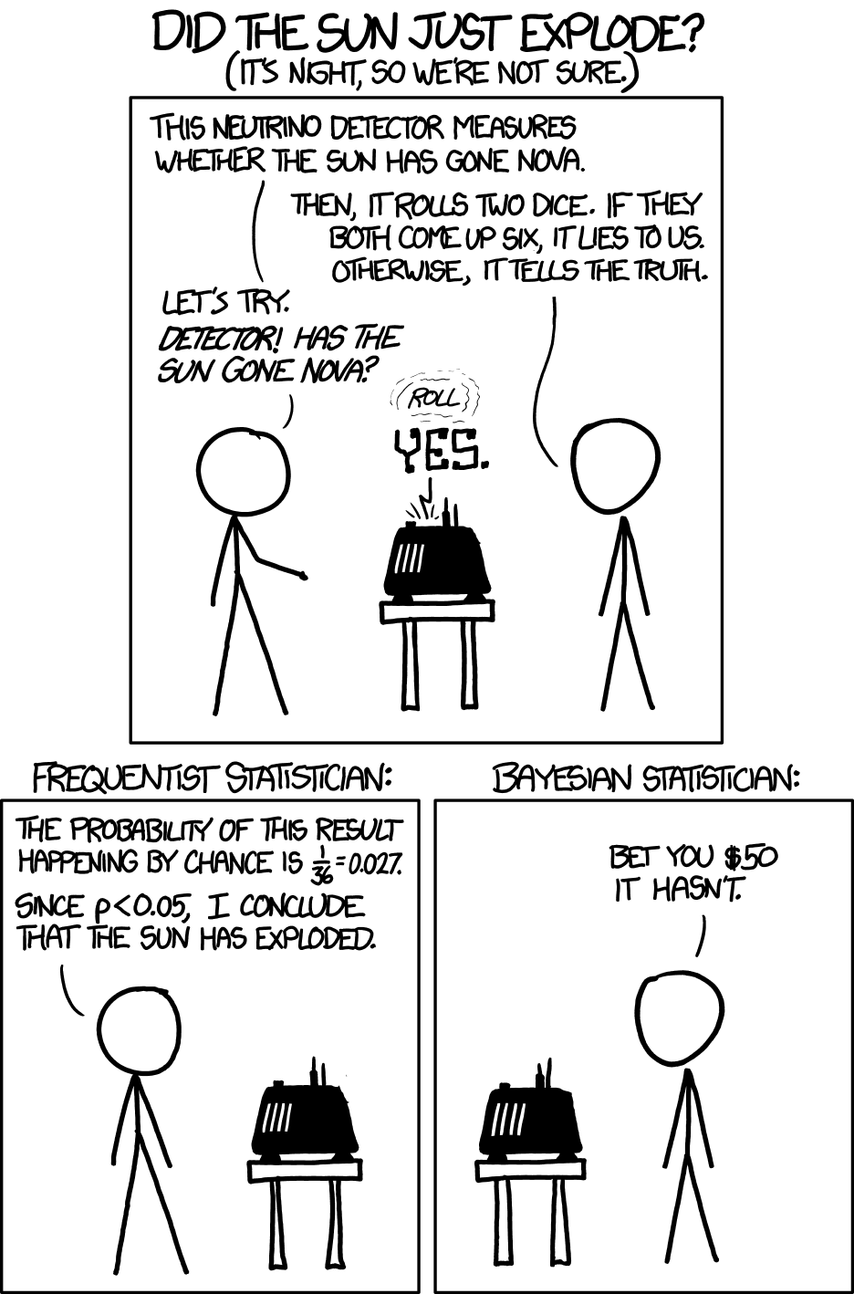
(mandatory strip from xkcd which appears in every discussion of Frequentists vs Bayesians)

---