I recently stumbled across a very interesting paper (thanks a lot, Noam!) titled “Auto-DeepLab: Hierarchical Neural Architecture Search for Semantic Image Segmentation”, by C. Liu et al.; the authors were able to find a network capable of state-of-the-art performance on a very hard problem, semantic image segmentation, in only 3 GPU days (with an NVIDIA Tesla P100). This is especially impressive since comparable methods require typically something like a thousand GPU days on the same hardware.

This sparked my interest in a very interesting technique called Differentiable Neural Architecture Search (DNAS). I decided to write a post about it to try to illustrate it in a simple way, and include links to the relevant literature in order to do a little service to readers who would like to start researching the topic.

If I had to sum up DNAS in one sentence, I would say that it is a technique which enables us to learn simultaneously the architecture of a neural network and its weights by transforming the NAS problem, typically discrete, into a continuous one, which can then be solved via gradient descent.

For definiteness, in the following I will show how DNAS can be applied to Convolutional Neural Networks (CNNs), but keep in mind that a lot of the concepts I will consider in the following can be effectively used for other architectures too.

Differentiable NAS and DARTS

In order to build a CNN, we typically need to specify its architecture first; this basically means choosing many parameters, like size/depth of each filter, which operations are applied on each layer, what is connected to what, and so on; for now, let us imagine we have encoded all this information in a vector of hyperparameters \(\alpha\).

Notice that for the kind of parameters I described, \(\alpha\) will contain only discrete variables; this can be quite problematic, because if we want to find the best architecture for a given problem we really want to solve the following nested optimization problem:

\[\begin{align} \min_\alpha \, &\mathcal{L}_{\text{val}}(\alpha, w^*(\alpha)) \tag{1}\\ \text{with } w^*(\alpha) &= \underset{w}{\operatorname{argmin}}\, \mathcal{L}_{\text{train}}(\alpha, w), \tag{2} \end{align}\]

where \(\mathcal{L}_{\text{val}}\) and \(\mathcal{L}_{\text{train}}\) are both the loss function calculated, respectively, on either a validation or a training set, and depend on the architecture of the network \(\alpha\) and on the weights \(w\). In other words, we want to find the architecture which, after being trained on a training set, gives the best results on a validation set.

Since \(\alpha\) is composed of discrete variables, Eq. (1) cannot be solved immediately via gradient descent. One could use reinforcement learning or evolutionary algorithms for Eq. (1), but notice that this entails training a large number of “useless” networks (via gradient descent on Eq. (2)), and this inner loop can be prohibitively time-consuming.

In the DARTS paper (by H. Liu et al.), the authors present a solution to this problem via continuous relaxation. This was not an entirely new idea (see “Convolutional Neural Fabrics” and “Connectivity Learning in Multi-Branch Networks”), but whereas previous approaches used it in order to fine tune specific parameters, like filter sizes and number of filters of a specific architecture, in DARTS the search space is made of cells with potentially highly complex topologies. Cells are then stacked to form the entire CNN.

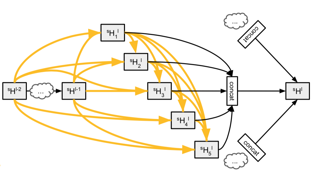
A cell is a directed acyclic graph, consisting of an ordered sequence of \(N\) nodes \(x^{(i)}\). Each node is associated with a tensor, and each directed edge \((i,j)\) (connecting node \(i\) to node \(j\)) is associated with some operation \(o^{(i,j)}\) on \(x^{(i)}\). Moreover, it is assumed that a cell has two tensors as inputs and one tensor as output; consistently with common choices for CNNs (see “Learning Transferable Architectures for Scalable Image Recognition”), the two tensors chosen as an input in DARTS are the outputs from the previous two cells. The output of a cell is found by applying a reduction operation (tipically concatenation) to all of the intermediate nodes. Thus, each node in a cell is given by

\[x^{(j)} = \sum_{i < j} o^{(i,j)}(x^{(i)}).\]

In order to transform the problem of architecture search to a continuous one, let us consider a set \(\mathcal{O}\) of operations, such as convolutions, dilated convolutions, max pooling, and zero (i.e., no connection). We can then parametrize \(o^{(i,j)}\) as

\[\bar{o}^{(i,j)}(x) = \sum_{o \in \mathcal{O}} \frac{ \exp(\alpha_o^{(i,j)}) }{ \sum_{o' \in \mathcal{O}} \exp(\alpha_{o'}^{(i,j)})} o(x),\]

i.e., we relax the choice of an operation via the softmax function.

The minimization problem in Eq. (1) can now be solved via gradient descent, since the \(\alpha\)s are now continuous. and the authors of DARTS propose to approximate the gradient with

\[\nabla_{\alpha} \mathcal{L}_{\text{val}}(\alpha, w^*(\alpha)) \approx \nabla_{\alpha} \mathcal{L}_{\text{val}}(\alpha, w - \xi \nabla_w \mathcal{L}_{\text{train}}(\alpha, w) , \tag{3}\]

where \(\xi\) assumes the role of an “inner optimization learning rate”. By applying the chain rule to the rightmost member of Eq. (3), it is possible to approximate the gradient at first order with

\[\nabla_\alpha \mathcal{L}_{\text{val}}(\alpha, w^*(\alpha)) \approx \nabla_\alpha \mathcal{L}_{\text{val}}(\alpha, w'),\]

where \(w' = w - \xi \nabla_w \mathcal{L}_{\text{train}}(\alpha, w)\).

Finally, the last step needed is to decode the architecture of the cell from the continuous set of \(\alpha\)s. A meaningful choice for CNNs is simply to retain, for each node, the two “strongest” operations connecting the node to the previous ones.

The global architecture of the network has to still be specified manually. In particular, the DARTS’ authors chose to search over two different kinds of cells: there are “normal” cells, where operations have stride one, and there are “reduction” cells, in which all the operations adjacent to the input nodes are of stride two. Then, as fairly common in networks built for image classification, the architecture is composed of many identical cells stacked on top of each other, except some specific points where the cells’ job is to downsample the incoming tensors.

This formulation of the problem of NAS is what made it possible for the authors of DARTS to find architectures capable of state-of-the-art performance in image classification in only a matter of a few GPU days.

Auto-Deeplab

A limitation of DARTS is the fact that it does not search for the best architecture at a network level: as written above, it only searches for the best cells in a given architecture, but the way to connect them has to be given from the start. Especially for tasks like semantic image segmentation, this is hard to know from the start; optimal architectures can be, in fact, very complicated.

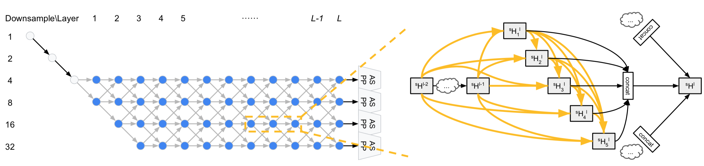(Auto-Deeplab search space; picture from their paper on arxiv)

With Auto-Deeplab, the search space is not only at the cell level, but also at the network level; this is done by considering a trellis of cells during training, and after that the final architecture is decoded via the Viterbi algorithm by keeping only the path with the strongest connections in the trellis.

Specifically, the authors restricted themselves to architectures where the first two layers are downsampling layers, and then each further layer can either keep the resolution of the incoming tensor, upsample it by 2, or downsample it by 2 (see the figure above). This search space is quite general, and includes as specific cases previously-found successful architectures, like DeepLabv3, Conv-Deconv, and Stacked Hourglass.

Another thing worth noticing is that the authors found empirically that it is better to start the optimization at the network level only after some epochs of optimization of the weights; if the architecture is optimized too early, it seems that networks tends to converge to some bad local optima.

The results of Auto-Deeplab on the Cityscapes dataset are the following:

Model	#Parameters	mIOU (%)
Auto-DeepLab-S	10.15M	79.74
Auto-DeepLab-M	21.62M	80.04
Auto-DeepLab-L	44.42M	80.33
DeepLabv3+	43.48M	79.55

(here, mIOU is the mean intersection over union).

It is worth noticing that the smallest architecture found by Auto-DeepLab is able to beat DeepLabv3+ with less than a fourth of the parameters! Similar results apply to other benchmarks as well.

Conclusion

The process of neural architecture search for now seems to me still very empirical, with a lot of important discoveries yet to be made which will allow us to tap the full potential of Deep Learning. I have the feeling that DNAS is one of the most promising approaches to this, and already since the time I started writing this article (I know, I am a slow writer) there have been multiple cool applications of DNAS which I cannot wait to learn a bit more about. For now, thanks for reading :-)