Time Series Forecasting with an LSTM Encoder/Decoder in TensorFlow 2.0
In this post
I want to illustrate a problem I have been thinking about in time series
forecasting, while simultaneously
showing how to properly use some Tensorflow features which greatly
help in this setting (specifically, the tf.data.Dataset class and Keras’
functional API).
Imagine the following: we have a time series, i.e., a sequence of values \(y(t_i)=y_i\) at times \(t_i\), and we also have at each time step some auxiliary features \(\boldsymbol{X}(t_i) = \boldsymbol{X}_i\) which we think are related with the values of \(y_i\). Some of the components of \(\boldsymbol{X}_i\) might be known for all times (think of them as predetermined features, like whether time \(t_i\) is a national holiday) whereas others are random and quite difficult to forecast in advance (say, the price of a Microsoft stock at time \(t_i\)).
If we want to train a model to forecast the future values of the time series we cannot use every feature, but rather we need to censor the features we would not be able to know at prediction time, as shown in the picture below.

For these kinds of tasks, a pretty straightforward procedure would be to use an autoregressive model of some kind (like ARMAX); these models allow us to take into account autocorrelations in a time series, and also can accept the deterministic features in the future (typically called “exogenous variables”). One limitation of ARMAX is that it is a linear model, and also one needs to specify the order of autocorrelations to be taken into account parametrically. LSTMs, instead, can learn nonlinear patterns, and are able to take into account autocorrelations in a nonparametric way!
So, let’s try this idea: let’s encode past observations in a latent space, and then use the encoded past as a sort of “context” to then perform forecasts with an LSTM1. In order to better illustrate this problem and my proposed solution, let’s consider in the following section a concrete example.
Example: Bike Sharing
Let’s start with a practical example of a time series and look at the UCI Bike Sharing Dataset; there we can find for each hour the amount of bikes rented by customers of a bike sharing service in Washington DC, together with other features such as whether a certain day was a national holiday, and which day of the week was it. The dataset can be downloaded with the following bash commands:
1
2
wget https://archive.ics.uci.edu/ml/machine-learning-databases/00275/Bike-Sharing-Dataset.zip
unzip Bike-Sharing-Dataset.zip -d bike_data
Our goal is to be able to predict the total bike usage for the week following prediction time. For the sake of simplicity, let’s skip a lot of data cleaning/feature engineering steps one should apply to this dataset, and just load it via the following:
1
2
3
4
5
6
7
8
9
10
11
12
13
14
15
16
17
18
19
20
21
22
23
24
25
26
27
28
29
30
31
32
33
34
35
36
37
38
39
40
41
42
43
44
45
46
47
48
49
50
import pandas as pd

df = pd.read_csv('bike_data/hour.csv', index_col='instant')

# Extracting only a subset of features
def select_columns(df):
    cols_to_keep = [
        'cnt',
        'temp',
        'hum',
        'windspeed',
        'yr',
        'mnth',
        'hr',
        'holiday',
        'weekday',
        'workingday'
    ]
    df_subset = df[cols_to_keep]
    return df_subset


# Some of the integer features need to be onehot encoded;
# but not all of them
def onehot_encode_integers(df, excluded_cols):
    df = df.copy()

    int_cols = [col for col in df.select_dtypes(include=['int'])
                if col not in excluded_cols]

    df.loc[:, int_cols] = df.loc[:, int_cols].astype('str')

    df_encoded = pd.get_dummies(df)
    return df_encoded

# cnt will be target of regression, but also a feature:
# it needs to be normalized. This is not the correct way to do it,
# as it leads to information leakage from test to training set.
def normalize_cnt(df):
    df = df.copy()
    df['cnt'] = df['cnt'] / df['cnt'].max()
    return df

# I <3 pandas pipes
dataset = (df
           .pipe(select_columns)
           .pipe(onehot_encode_integers,
                 excluded_cols=['cnt'])
           .pipe(normalize_cnt)
           )
As mentioned before, we want to feed the “past” plus some deterministic features in the future to a Keras model and get back a forecast; in order to make Keras accept this data, it has to be reshaped in an appropriate way. We need to split it into “windows” where each row is a time step and each column correspond to a feature. Moreover, if we want to split the training into multiple batches we need to aggregate all these windows in a tensor of shape \((n_{batches}, n_{timesteps}, n_{features})\).
Since the dataset is already loaded in a Pandas DataFrame, we could easily do these steps with a mix of Pandas
methods (DataFrame.rolling() & co.) and then transform the data into Numpy arrays
(which TensorFlow can then ingest).
I try to show here an approach I like more, that can work seamlessly for much larger datasets
which do not fit in memory and has a very clean API: we initialize a tf.data.Dataset object from the
data and then transform it via TensorFlow builtin functions. So, we can just define a function that
returns the desired form of the dataset like this:
1
2
3
4
5
6
7
8
9
10
11
12
13
14
15
16
17
18
19
20
21
22
23
24
def create_dataset(df, n_deterministic_features,
                   window_size, forecast_size,
                   batch_size):
    # Feel free to play with shuffle buffer size
    shuffle_buffer_size = len(df)
    # Total size of window is given by the number of steps to be considered
    # before prediction time + steps that we want to forecast
    total_size = window_size + forecast_size

    data = tf.data.Dataset.from_tensor_slices(df.values)

    # Selecting windows
    data = data.window(total_size, shift=1, drop_remainder=True)
    data = data.flat_map(lambda k: k.batch(total_size))

    # Shuffling data (seed=Answer to the Ultimate Question of Life, the Universe, and Everything)
    data = data.shuffle(shuffle_buffer_size, seed=42)

    # Extracting past features + deterministic future + labels
    data = data.map(lambda k: ((k[:-forecast_size],
                                k[-forecast_size:, -n_deterministic_features:]),
                               k[-forecast_size:, 0]))

    return data.batch(batch_size).prefetch(tf.data.experimental.AUTOTUNE)
Notice that aside from extracting windows out of the dataset and selecting the correct portions out
of them, we also randomize the order of training examples we show to the model, batch it, and
prefetch it.
Via the generate_dataset function we can create tf.data.Dataset objects
to feed to TensorFlow:
1
2
3
4
5
6
7
8
9
10
11
12
13
14
15
16
17
18
19
20
21
22
23
24
25
26
27
28
29
30
31
32
33
34
35
36
37
38
39
40
41
# Times at which to split train/validation and validation/test
val_time = 10000
test_time = 14000

# How much data from the past should we need for a forecast?
window_len = 24 * 7 * 3  # Three weeks
# How far ahead do we want to generate forecasts?
forecast_len = 24 * 5  # Five days

# Auxiliary constants
n_total_features = len(dataset.columns)
n_aleatoric_features = len(['cnt', 'temp', 'hum', 'windspeed'])
n_deterministic_features = n_total_features - n_aleatoric_features

# Splitting dataset into train/val/test
training_data = dataset.iloc[:val_time]
validation_data = dataset.iloc[val_time:test_time]
test_data = dataset.iloc[test_time:]


# Now we get training, validation, and test as tf.data.Dataset objects

batch_size = 32

training_windowed = create_dataset(training_data,
                                   n_deterministic_features,
                                   window_len,
                                   forecast_len,
                                   batch_size)

validation_windowed = create_dataset(validation_data,
                                     n_deterministic_features,
                                     window_len,
                                     forecast_len,
                                     batch_size)

test_windowed = create_dataset(test_data,
                               n_deterministic_features,
                               window_len,
                               forecast_len,
                               batch_size=1)
This kind of train/cv/test split is most likely quite biased (as I already wrote in another article on my blog), but for the sake of simplicity let’s keep it this way.
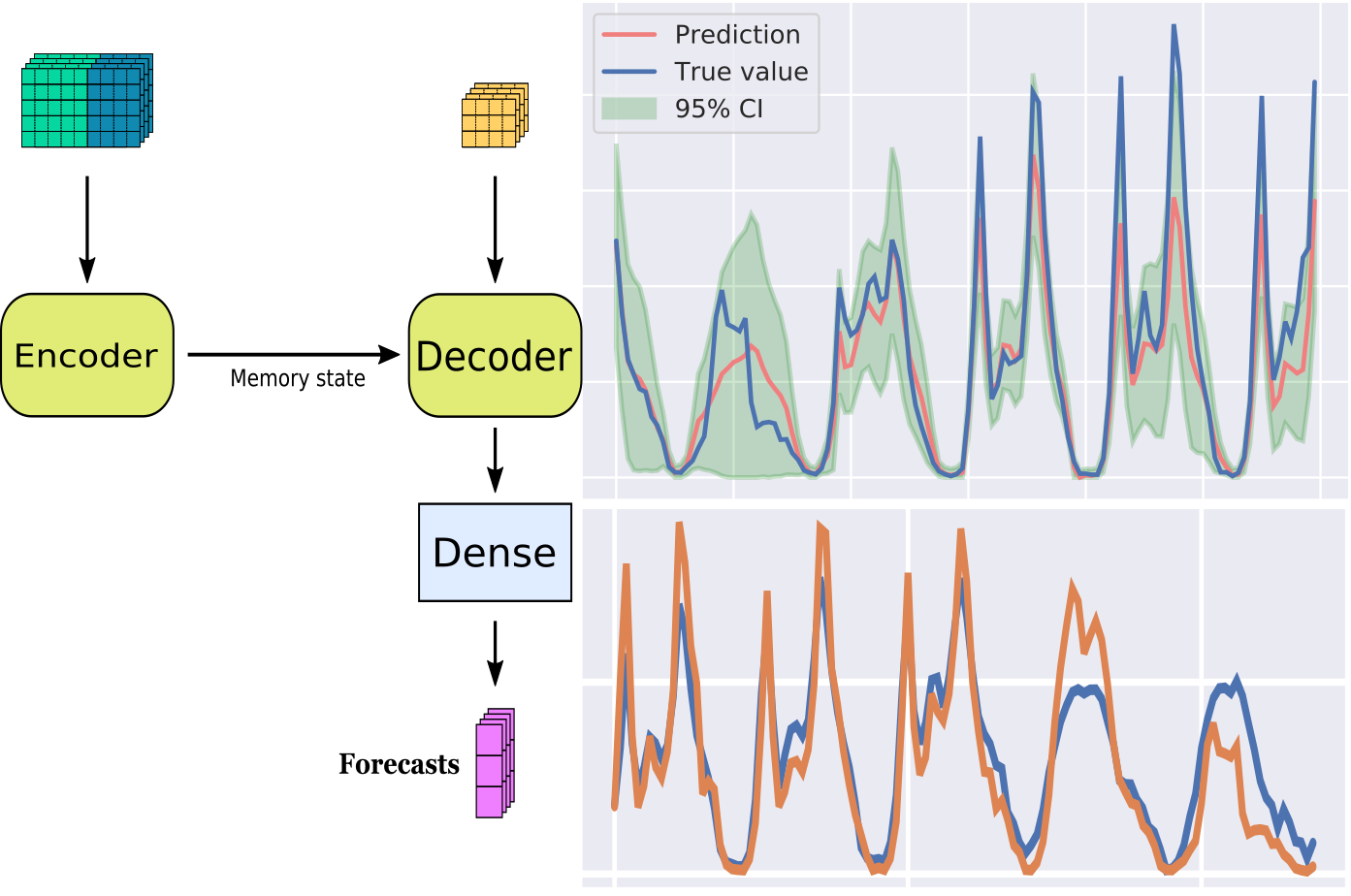
Now that the data is prepared, we need to define the model. The specifics of the neural architecture I am using here are not particularly optimized, but they follow from the basic idea that I want to encode past observations in a latent space, and then use the encoded past as a sort of “context” to then perform forecasts with an LSTM.

Thus, we can define the model pictured above via the Keras functional API as follows:
1
2
3
4
5
6
7
8
9
10
11
12
13
14
15
16
17
18
19
20
21
22
23
24
25
26
27
28
import tensorflow as tf

latent_dim = 16

# First branch of the net is an lstm which finds an embedding for the past
past_inputs = tf.keras.Input(
    shape=(window_len, n_total_features), name='past_inputs')
# Encoding the past
encoder = tf.keras.layers.LSTM(latent_dim, return_state=True)
encoder_outputs, state_h, state_c = encoder(past_inputs)

future_inputs = tf.keras.Input(
    shape=(forecast_len, n_deterministic_features), name='future_inputs')
# Combining future inputs with recurrent branch output
decoder_lstm = tf.keras.layers.LSTM(latent_dim, return_sequences=True)
x = decoder_lstm(future_inputs,
                 initial_state=[state_h, state_c])

x = tf.keras.layers.Dense(16, activation='relu')(x)
x = tf.keras.layers.Dense(16, activation='relu')(x)
output = tf.keras.layers.Dense(1, activation='relu')(x)

model = tf.keras.models.Model(
    inputs=[past_inputs, future_inputs], outputs=output)

optimizer = tf.keras.optimizers.Adam()
loss = tf.keras.losses.Huber()
model.compile(loss=loss, optimizer=optimizer, metrics=["mae"])
In order to train the model, since we are using tf.data.Dataset objects for the data,
we just need to call
1
2
history = model.fit(training_windowed, epochs=25,
                    validation_data=validation_windowed)
We can check for the mean squared error on the test set by calling model.evaluate(test_windowed)
and we obtain for these Hyperparameters a mean absolute error of about
\(75\) bikes; not too bad! Some sample forecasts are pictured below, compared with the
actual number of bikes in use after prediction time.

Bonus: What if we want to forecast probability distributions?
As I previously argued on my blog, point predictions are not the full story, and it is often of uttermost importance to be able to predict probability distributions2. Luckily, since we built our model with TensorFlow, we can just make a slight modification to the head of the neural network and attach to it a TensorFlow Probability distribution layer; thus, we can define the model via
1
2
3
4
5
6
7
8
9
10
11
12
13
14
15
16
17
18
19
20
21
22
23
24
25
26
27
import tensorflow_probability as tfp

tfd = tfp.distributions

# First branch of the net is an lstm which finds an embedding for the past
past_inputs = tf.keras.Input(
    shape=(window_len, n_total_features), name='past_inputs')
# Encoding the past
encoder = tf.keras.layers.LSTM(latent_dim, return_state=True)
encoder_outputs, state_h, state_c = encoder(past_inputs)

future_inputs = tf.keras.Input(
    shape=(forecast_len, n_deterministic_features), name='future_inputs')
# Combining future inputs with recurrent branch output
decoder_lstm = tf.keras.layers.LSTM(latent_dim, return_sequences=True)
x = decoder_lstm(future_inputs,
                 initial_state=[state_h, state_c])
x = tf.keras.layers.Dense(8, activation='relu')(x)
x = tf.keras.layers.Dense(8, activation='relu')(x)
x = tf.keras.layers.Dense(2, activation='relu')(x)
output = tfp.layers.DistributionLambda(
    lambda t: tfd.Normal(loc=t[..., 0],
                         scale=0.01*tf.math.softplus(t[..., 1])),
    name='normal_dist')(x)

model = tf.keras.models.Model(
    inputs=[past_inputs, future_inputs], outputs=output)
The loss function now cannot be MSE or Huber anymore, because the model returns distributions. A natural choice here is to do maximize likelihood, which is equivalent to minimizing negative log-likelihood. So, the model can be trained in the following way:
1
2
3
4
5
6
7
8
9
10
def negloglik(y, p_y): return -p_y.log_prob(y)


optimizer = tf.keras.optimizers.Adam(lr=0.001)
model.compile(loss=negloglik,
              optimizer=optimizer)

history = model.fit(training_windowed,
                    epochs=25,
                    validation_data=validation_windowed)
And after a while we can obtain reasonable-looking forecasts.

Explainability of the model
Well, that’s a topic for another day :-)
Conclusion
This was just a very simple application; I did not optimize the model at all, but I think one can build upon this to achieve interesting results. Especially, better data cleaning and feature engineering would help a lot. It would be interesting to see whether with better hyperparameters we can obtain much better performance.
Still, I think this code exemplifies how easy it has become nowadays to build not-so-trivial neural networks (like the one we had here, combining LSTMs and probabilistic layers) and train them. Modern frameworks really do abstract a lot of the heavy lifting for us!
The full code used for this post can be found on this Google Colab notebook.
-
This kind of technique is very common in machine translation; see this tutorial for a nice introduction. ↩
-
I recently read a very accessible book on the problems which can arise in businesses when ignoring probability distributions which I wish more people would read and understand. It is called The Flaw of Averages, by Sam L. Savage, and I wholeheartedly recommend it :-) ↩