Graphs are awesome, hypergraphs are hyperawesome! Hypergraphs are a generalization of graphs where one relaxes the requirement for edges to connect just two nodes and allows instead edges to connect multiple nodes. They are a very natural framework in which to formulate and solve problems in a wide variety of fields, ranging from genetics to social sciences, physics, and more! But whereas for manipulating and visualizing graphs there are many mature Python libraries, the same cannot be said for hypergraphs.

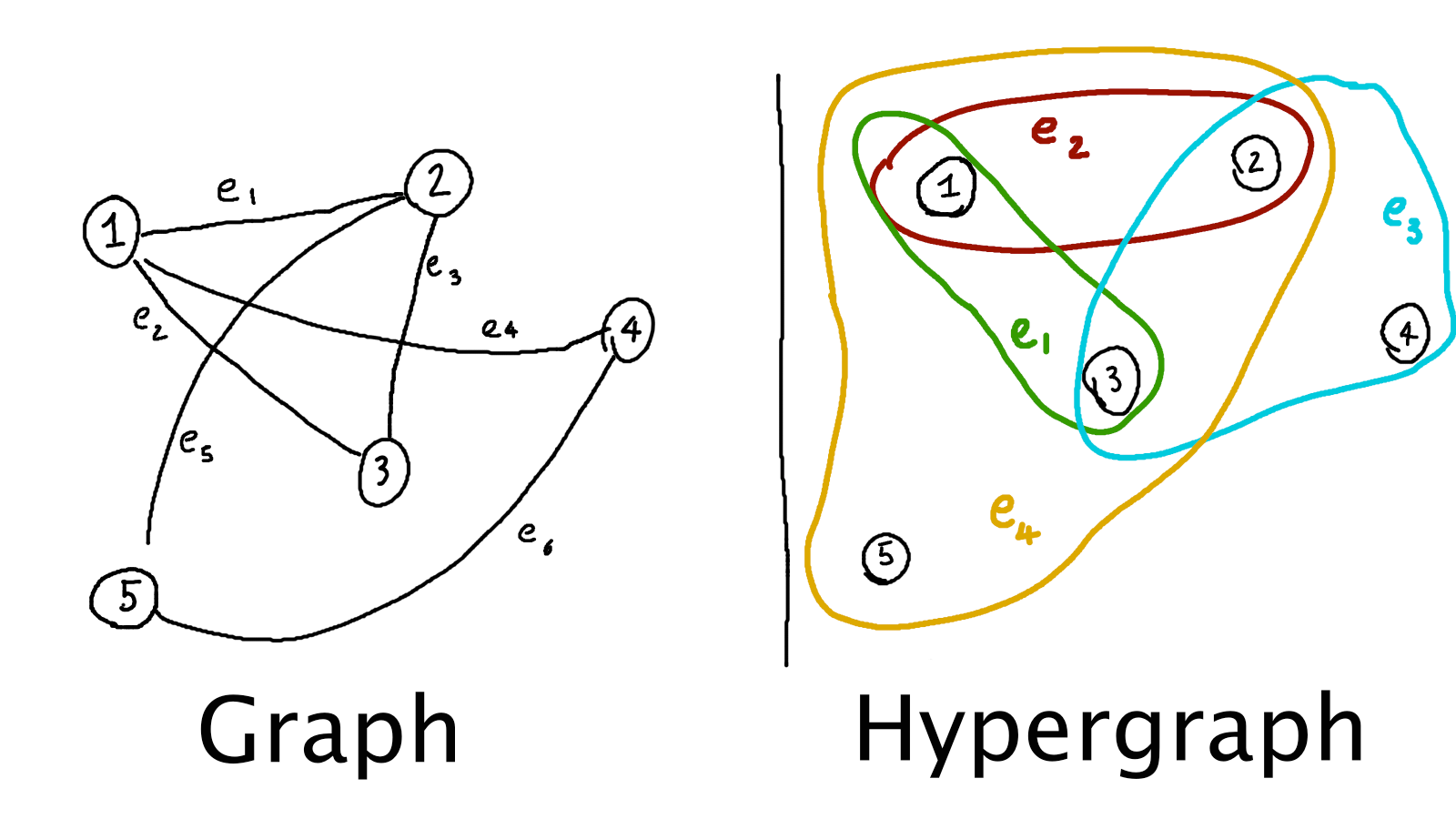
I recently needed to visualize some hypergraphs and could not find any library which satisfied me; moreover, as far as I could see, all of them were representing hypergraphs via Euler diagrams (i.e., like the hand-drawn hypergraph above). Unfortunately this method was not producing good plots for my use case; what I ended up doing was to represent a hypergraph as a collection of graphs, and plotting them via the awesome networkx library.

I decided to write about my approach to plotting hypergraphs, as it produces quite interesting plots for the kind of data I am looking at lately (essentially Ising models, but containing many body interactions too), and, with some adaptations, it could be of some help to others struggling with hypergraph visualization tasks.

First ideas and attempts

We will start by representing a hypergraph in Python with the following code: Notice that this is just a very basic way to do so, as edges should really be Python frozensets, so that a collection of them can also be a set, and the node set should also be a frozenset or a set. A better schema would help us greatly in case we were developing a library for hypergraph algorithms, but in this post I decided to keep the simple schema above for the sake of simplicity.

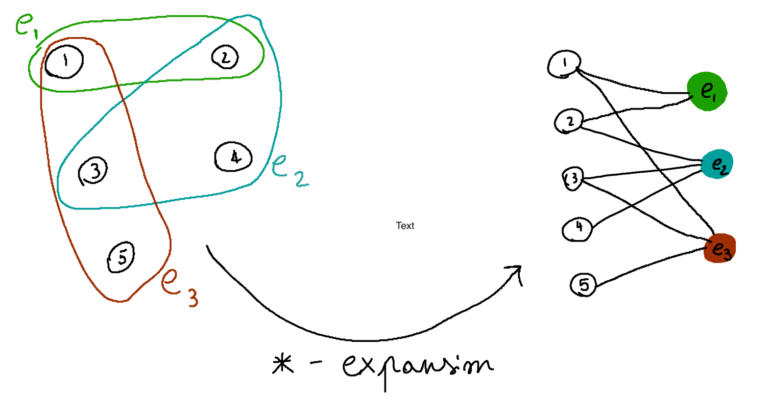
We can start by noticing that any hypergraph can be transformed into a graph via the so-called star expansion, i.e., we create a new graph having as node set both the nodes and the edges of the original hypergraph, and the edges are given by the incidence relations in the original hypergraph (if a node \(n\) was part of an edge \(e\) in the hypergraph, there should be an edge between \(n\) and \(e\) in the new graph).

This is way less complicated than it sounds, as shown in the picture below:

In many applications plotting the star expansion of a hypergraph might be enough. For example, the star expansion of test_hypergraph (defined above) looks as follows

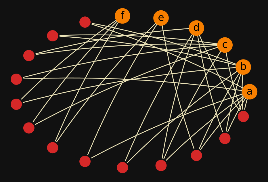
By making some edits, such as expanding only the edges connecting three or more nodes and choosing a different layout for the extra nodes, one can also plot test_hypergraph like this:

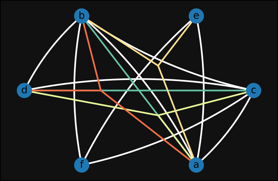
In the plot above we can read, for instance, the edge (a,b,d) from the three red lines connecting a, b, and d.

While the fewer extra nodes caused by a partial star expansion make the second plot slightly more readable, both of the plots above are still deeply unsatisfying. My main issues with these visualizations (and similar ones I ended up producing while experimenting on this topic) are the following:

1. There is too much information on a single image, and far too many overlapping lines; this makes the plot hard to read, and potentially useless.
2. The embeddings one can choose to plot graphs can significantly help in understanding the structure of the graph itself; by doing a star expansion this is in general not the case anymore, as nodes are intermixed with hyperedges.

Solving #2 is very challenging, and most likely heavily dependant on the kind of hypergraph one wants to visualize. I found a strategy which works quite well for solving #1 in case it makes sense to split the edges of a hypergraph by their cardinality, and will explain my approach below.

Decomposing a hypergraph into many graphs

The key idea is that we will decompose the edges of a hypergraph by how many nodes they contain, in a way completely analogous to how physicists speak of 2-body interactions, 3-body interactions, and so on, and plot these different “components” of the hypergraph separately.

To decompose the edge set of a hypergraph (assuming a schema like the one we used for test_hypergraph above) by the edges’ cardinality, we can write For instance, the decomposed_edges dictionary for test_hypergraph looks as follows

1
2
3
4
5
6
7
{
  2: [('a', 'b'), ('b', 'c'), ('c', 'd'), ('a', 'c'),
      ('b', 'f'), ('f', 'c'), ('e', 'f'), ('a', 'e'),
      ('b', 'd')],
  3: [('a', 'c', 'd'), ('a', 'b', 'e'), ('a', 'b', 'd')],
  4: [('a', 'b', 'c', 'd')]
}

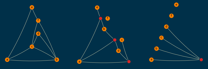
So then, we can try to plot, for each edge order \(i\), the star expansion of the hypergraph given by the node set of the original graph, together with the edge set decomposed_edges[i] (except for \(i = 2\), where we will just plot the graph without star expanding it), and see what it looks like. The code to achieve this is the following:

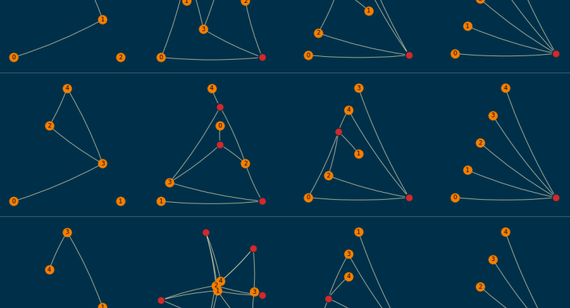
Applying the plot_hypergraph_components function to test_hypergraph produces the following plot:

This script should be pretty straightforward, but let me know if you want anything clarified further. One weird choice I had to make is to let g be a networkx.DiGraph, as I was not able to draw curvy lines via the connectionstyle argument if g was instead a networkx.Graph.

The fact that the red nodes (which are the extra nodes obtained by star expansion) have always the same order in each subplot makes this plot very easy to read. It is still not perfect, but arguably much more readable than our earlier attempts. For instance, it is obvious from the rightmost subplot that there is only one edge of order 4, and it is (a,b,c,d), and from the subplot in the middle it is easy to see that the only edges of order 3 are (a,b,e), (a,b,d), and (a,c,d).

Other examples with random hypergraphs

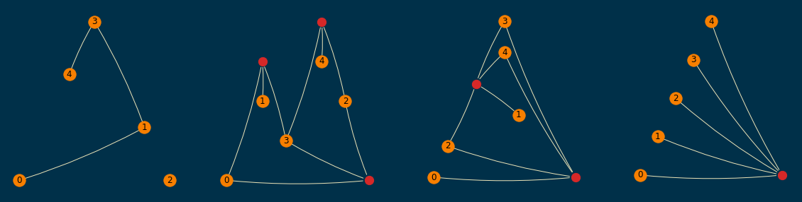
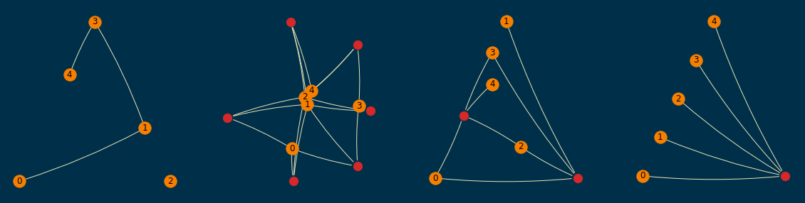
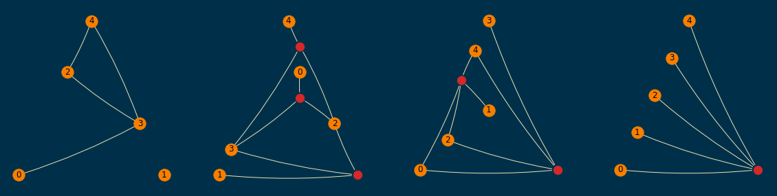
We can also generate some random hypergraphs by starting with a set of nodes and adding edges at random between them, until we reach a specified number of them, i.e.,

A sample of them (order=5 and size=10) is shown below; empirically, I found them to be readable enough, even when a planar layout was not achievable.

Conclusion

The procedure illustrated above can be quite helpful in plotting hypergraphs via networkx. Especially in contexts such as quantum physics, statistical mechanics, and so on, where the order of a hyperedge matters, this could be a helpful visualization.

A drawback of the proposed scheme could be that in each of the subplots the position of the nodes can vary in general; this could be trivially solved by arbitrarily fixing the pos argument in the code for plot_hypergraph_components, but maybe problem-specific properties can help in making a meaningful choice for it.

If you made it this far, thanks for reading :-)