Borwein Integrals interpreted via Path Integrals

The ability to see common patterns and analogies, to conjecture universal laws starting from the particular things we can experience, is a powerful tool, which arguably is one of the foundations of science. Although we rely constantly on our inductive abilities, the cases when our intuition is spectacularly wrong teaches us valuable lessons, in the same way optical illusions can make us understand how our visual perception works.

My favorite example about this is the (apparent) pattern one can see in Borwein integrals (from the father and son who popularized this kind of integrals, in [Borwein and Borwein, 2001] ); my interest in them was rekindled by a very cool recent article by Majumdar and Trizac, where they link the strange properties of Borwein integrals to probability distributions associated with some random walks, and with an argument essentially about causality they are able to explain what is happening “under the hood”.

Let’s then start our study of these interesting integrals. With just a tiny bit of effort, it is easy to prove that

\int_{- \infty}^{\infty} d x s i n c (x) = π

and with some more patience, one can also prove that

\begin{aligned} \int_{- \infty}^{\infty} d x s i n c (x) s i n c (x / 3) & = π \\ \int_{- \infty}^{\infty} d x s i n c (x) s i n c (x / 3) s i n c (x / 5) & = π \\ \dots \\ \int_{- \infty}^{\infty} d x s i n c (x) s i n c (x / 3) \dots s i n c (x / 13) & = π \end{aligned}

Wow, there seems to be a pattern here, and one could maybe conjecture a handful of reasons why all these kinds of integrals must be equal to $π$ .

The plot thickens after a Maple developer was playing with this kind of integrals and he noticed that

\int_{- \infty}^{\infty} d x s i n c (x) s i n c (x / 3) \dots s i n c (x / 15) \approx π - 4.6 \times 10^{- 11} < π,

i.e., the value of the integral is slightly less than $π$ . While at first he attributed this problem to a bug in the code, indeed after a few days he realized that this is indeed the correct result. There are various papers about the calculation and interpretation of this kind of integrals ([Borwein and Borwein, 2001], [Schmid, 2014]), but the one which in my opinion is most intuitive and has potential for generalization is the above-mentioned [Majumdar and Trizac, 2019], where they link Borwein integrals to random walks. Heavily borrowing from [Majumdar and Trizac, 2019], I will explain what is happening under the hood of these integrals with the tool that I think makes essentially any kind of random process very clear (especially to physicists): the path integral.

Interpretation via a Path Integral

Let’s start from a seemingly unrelated¹ problem: consider a particle which starts at $x_{0} = 0$ and that moves at discrete time steps by performing a sequence of (uniformly distributed) random jumps, i.e.,

x_{i} = x_{i - 1} + δ_{i},

where $x_{i}$ is the position of the particle at the $i$ -th time, and $δ_{i}$ is a random variable uniformly distributed between $- a_{i}$ and $a_{i}$ (assume $a_{i} > 0$ ). Notice that, although the change in the position due to each jump is always uniformly distributed, the parameters of the uniform distribution are allowed to change between jumps; in particular, the maximum distance that can be jumped with the first jump is $a_{1}$ , with the second one is $a_{2}$ , and so on.

At any point in time, the state of the particle can be in general associated with the probability density of finding the particle at a certain position $x$ ; therefore, states of this system live in the vector space of integrable functions on the real axis. I will use the bra-ket notation, and write then elements of this vector space as $| ϕ ⟩$ , scalar products as

⟨ ϕ | ψ ⟩ = \int_{R} d x ϕ (x) ψ (x) .

States labeled by positions, like $x$ and $x_{i}$ , are states where we are definitely sure that the particle occupies a certain position, and are essentially Dirac deltas $δ (. . .)$ , i.e.,

⟨ \bar{x} | ψ ⟩ = \int_{R} d x δ (x - \bar{x}) ψ (x) = ψ (\bar{x}),

and we can easily prove that they satisfy the completeness relation:

\int_{R} d \tilde{x} ⟨ ϕ | \tilde{x} ⟩ ⟨ \tilde{x} | ψ ⟩ = \int_{R} d \tilde{x} \int_{R} d x_{1} \int_{R} d x_{2} ϕ (x_{1}) δ (x_{1} - \tilde{x}) δ (x_{2} - \tilde{x}) ψ (x_{2}) = ⟨ ϕ | ψ ⟩,

for any pair of vectors ${| ϕ ⟩, | ψ ⟩}$ .

We can associate to each jump an operator $\hat{S} (a)$ in the following way: suppose that at some generic point in time the probability density for the position $x$ of the particle is $p_{i} (x) = ⟨ x | ϕ ⟩;$ after a random jump of maximum size $a > 0$ , the distribution will in general be given by another state, which we will define to be $\hat{S} (a) | ϕ ⟩$ . The resulting probability density will then be $p_{i + 1} (x) = ⟨ x | \hat{S} (a) | ϕ ⟩ .$

The time evolution of the system can then be obtained by repeated application of the operator $\hat{S} (a)$ . Therefore, the pdf for the position of the particle after $N$ steps is

p_{N} (x) = ⟨ x | \hat{S} (a_{N}) \hat{S} (a_{N - 1}) \dots \hat{S} (a_{1}) | x_{0} = 0 ⟩;

by introducing completeness relations between each pair of operators we obtain

p_{N} (x) = \int_{R^{N - 1}} d x_{1} \dots d x_{N - 1} ⟨ x | \hat{S} (a_{N}) | x_{N - 1} ⟩ ⟨ x_{N - 1} | \hat{S} (a_{N - 1}) | x_{N - 2} ⟩ \dots ⟨ x_{1} | \hat{S} (a_{1}) | x_{0} = 0 ⟩ .

Notice that all of the factors appearing in the equation above are quite trivial to calculate, as in them $\hat{S}$ acts only on states where the particle is for sure at a specific point. This should not be surprising, as it is essentially a manifestation of the chain rule for independent events. Therefore we have

⟨ x_{i} | \hat{S} (a) | x_{i - 1} ⟩ = U_{x_{i - 1} - a}^{x_{i - 1} + a} (x_{i}) = U_{- a}^{+ a} (x_{i} - x_{i - 1}),

where we introduced for the continuous uniform distribution the symbol

U_{a}^{b} (x) = {\begin{cases} \frac{1}{b - a}, & i f a \leq x \leq b \\ 0 & o t h e r w i s e \end{cases}

and so we can write

p_{N} (x) = \int_{R^{N - 1}} d x_{1} \dots d x_{N - 1} U_{- a_{N}}^{+ a_{N}} (x - x_{N - 1}) U_{- a_{N - 1}}^{+ a_{N - 1}} (x_{N - 1} - x_{N - 2}) \dots U_{- a_{1}}^{+ a_{1}} (x_{1}) .

By noticing that the Fourier transform of the uniform distribution is

\int_{R} d x U_{- a_{i}}^{+ a_{i}} (x) e^{- i k x} = s i n c (a_{i} k),

and that according to the Convolution Theorem convolutions are mapped to products, we obtain

p_{N} (x) = \int_{R} \frac{d k}{2 π} \prod_{i = 1}^{N} s i n c (a_{i} k) e^{- i k x},

And so, in order to calculate the Borwein integrals we were originally interested in we just need to calculate

2 π p_{N} (0) = \int_{R} d k \prod_{i = 1}^{N} s i n c (a_{i} k),

which in the “path-integral” picture we developed above means we need to integrate only over paths which start from the origin and, after $N$ steps, end up being in the origin again.

Now, let’s ask ourselves the following question: what happens if we perform the substitution

U_{- a_{1}}^{+ a_{1}} (x_{1}) ⟶ \frac{1}{2 a_{1}},

i.e., if we forget that the first step of our particle was bounded in size by $a_{1}$ ? Sure, we will be introducing some “spurious” paths in the path integral, but then we could write $p_{N} (0)$ as

\begin{matrix} p_{N} (0) "=" \int_{- \infty}^{\infty} d x_{N - 1} U_{- a_{N}}^{a_{N}} (- x_{N - 1}) \int_{- \infty}^{\infty} d x_{N - 2} U_{- a_{N - 1}}^{a_{N - 1}} (x_{N - 1} - x_{N - 2}) \int_{- \infty}^{\infty} d x_{N - 3} \dots \\ \dots \int_{- \infty}^{\infty} d x_{1} U_{- a_{2}}^{a_{2}} (x_{2} - x_{1}) \frac{1}{2 a_{1}} \end{matrix}

(where we put the equal sign between quotation marks to higlight the fact that this is not true in general). Notice then that the integral over $d x_{1}$ is equal to $1$ , independent of $x_{2}$ ; therefore also the integral over $d x_{2}$ is unity, and so on, so that we simply have

p_{N} (0) "=" \frac{1}{2 a_{1}} .

The question then becomes: when is this result correct (i.e., when can we omit the ugly quotation marks in the formula above)?

The spurious paths we effectively introduced with our procedure are the ones for which $x_{1} > a_{1}$ . But suppose that

a_{1} > \sum_{i = 2}^{N} a_{i};

in this case, the spurious paths cannot contribute to $p_{N} (0)$ , as even if the particle would jump in the direction of the origin at each step, the jump sizes after the first one would be bounded by the $a_{i}$ s, and could arrive at most at a distance

| x_{1} | - \sum_{i = 2}^{N} a_{i} > 0

away from the origin. In some way, one can interpret this as a sort of causal argument: if the information that $U_{- a_{1}}^{+ a_{1}} (x)$ has a boundary cannot reach the origin in $N$ steps, the probability density at the origin will be constant and invariant with $N$ as the time steps. When “spurious” paths are able to backtrack to the origin, the value of the probability density must become strictly smaller as, in a way, it would stay constant only by adding the (positive) contribution of the “spurious” paths. Therefore, for Borwein integrals, we do have that

\begin{aligned} \frac{1}{3} + \frac{1}{5} + \dots + \frac{1}{13} \approx 0.955 < 1 \\ ⟹ \int_{- \infty}^{\infty} d x s i n c (x) s i n c (x / 3) \dots s i n c (x / 13) = 2 π p_{N} (0) = π, \end{aligned}

but also, when the information about the boundedness of the first jump reaches the origin, that

\begin{aligned} \frac{1}{3} + \frac{1}{5} + \dots + \frac{1}{15} \approx 1.022 > 1 \\ ⟹ \int_{- \infty}^{\infty} d x s i n c (x) s i n c (x / 3) \dots s i n c (x / 15) < π . \end{aligned}

Generalizations

Notice how the initially given form of Borwein integrals, with odd integers appearing in the arguments of $s i n c$ functions, was just smoke and mirrors: we could have chosen any sequence of $a_{i}$ s, provided that

a_{1} > \sum_{i = 2}^{N} a_{i},

and the value of the integral would still be $π / a_{1}$ . Therefore, from the proof above, we might as well state that

\int_{- \infty}^{\infty} d x \prod_{i = 1}^{N} s i n c (a_{i} x) = π, a_{1} > \sum_{i = 2}^{N} a_{i}, a_{i} \in R^{+} .

In our proof also we never made use of the fact that the probability distribution of jumps after the first one was uniform: we just needed them to have finite support and to be correctly normalized. So, for instance, as the Fourier transform of Bessel functions of integer order $α$ divided by their argument to the power of $α$ satisfy these properties, we can also find the following nontrivial identities for Bessel functions:

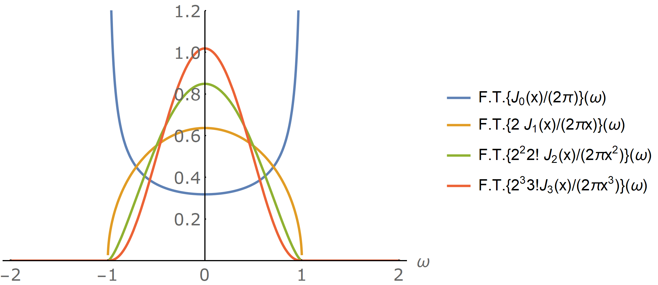
\int_{- \infty}^{\infty} d x s i n c (a_{1} x) \prod_{i = 2}^{N} \frac{2^{i} i! J_{α} (a_{i} x)}{2 π (a_{i} x)^{α}} = π, a_{1} > \sum_{i = 2}^{N} a_{i}, a_{i} \in R^{+}, α \in N .

Fourier transforms of Besse

…Or we can even get more general ones by mixing Bessel functions of different order: in the random walk picture, that would amount to allowing jumps after the first one to be characterized by the Fourier transform of the corresponding factor.

Even more, by considering discrete jumps instead of continuously-distributed ones, one can introduce other trigonometric functions in the integrands. In [Majumdar and Trizac, 2019], they even find identities for multi-dimensional integrals and for other interesting mathematical problems, such as proving when

\int_{- \infty}^{+ \infty} d k \prod_{i = 1}^{N} f_{i} (a_{i} k) \overset{?}{=} \sum_{k = - \infty}^{+ \infty} \prod_{i = 1}^{N} f_{i} (a_{i} k),

by only using causal reasoning.

Conclusion

I think I finally understood what is happening with Borwein integrals, and their connection with random walks is deeply interesting in my opinion. The fact that the probability distribution is affected by boundary effects (i.e, from the fact that the density is not constant over all the real numbers) only when information from the boundary is carried by some paths is a great idea, and for sure can be applied way beyond Borwein integrals.

If you liked this post, I think a great thing to see next is the talk “When random walkers help solving intriguing integrals”, by E. Trizac. For now, thanks a lot for reading!

Keeping in mind that the $s i n c$ function is the Fourier transform of the rectangular function (and therefore of the continuous uniform distribution), and that products are mapped to convolutions when Fourier-transformed, you might already see that this problem is not so unrelated after all! ↩

30 Aug 2020

« Data science case studies: easy to avoid common mistakes Should employees be promoted at random? Science says: “IDK, maybe?” »

Alessandro Angioi

Borwein Integrals interpreted via Path Integrals

Interpretation via a Path Integral

Generalizations

Conclusion

Explore →